OpenCV: Color-spaces and splitting channels
06 Nov 2014
There are more than 150 color-space conversion methods available in OpenCV. It is very easy to convert from one to another. We’re going to see how to do that and how to see what these color-spaces and its channels looks like. Watch the video to see how to change color-spaces and split channels using OpenCV.
Pre-requirements:
- OpenCV installed: How to install OpenCV 3 on Ubuntu
Introduction
We can say that a color-space is a combination of a color model and a mapping function (this definition is well-known). For color model, we can understand any mathematical model that can be used to represent colors as numbers (e.g. RGB(255, 0, 0) represents the red color). For mapping function, we can understand any function that can map a color model to an absolute color space, in order to connect this color system to the real world, making it usable.
Conversion between color-spaces
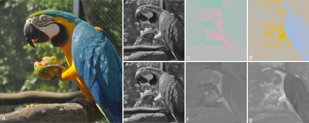
Our goal here is to visualize each of the three channels of these color-spaces: RGB, HSV, YCrCb and Lab. In general, none of them are absolute color-spaces and the last three (HSV, YCrCb and Lab) are ways of encoding RGB information. Our images will be read in BGR (Blue-Green-Red), because of OpenCV defaults. For each of these color-spaces there is a mapping function and they can be found at OpenCV cvtColor documentation.
One important point is: OpenCV imshow() function will always assume that the Mat shown is in BGR color-space. Which means, we will always need to convert back to see what we want. Let’s start.
HSV
While in BGR, an image is treated as an additive result of three base colors (blue, green and red), HSV stands for Hue, Saturation and Value (Brightness). We can say that HSV is a rearrangement of RGB in a cylindrical shape. The HSV ranges are:
- 0 > H > 360 ⇒ OpenCV range = H/2 (0 > H > 180)
- 0 > S > 1 ⇒ OpenCV range = 255*S (0 > S > 255)
- 0 > V > 1 ⇒ OpenCV range = 255*V (0 > V > 255)
YCrCb or YCbCr
It is used widely in video and image compression schemes. The YCrCb stands for Luminance (sometimes you can see Y’ as luma), Red-difference and Blue-difference chroma components. The YCrCb ranges are:
- 0 > Y > 255
- 0 > Cr > 255
- 0 > Cb > 255
Lab
In this color-opponent space, L stands for the Luminance dimension, while a and b are the color-opponent dimensions. The Lab ranges are:
- 0 > L > 100 ⇒ OpenCV range = L*255/100 (1 > L > 255)
- -127 > a > 127 ⇒ OpenCV range = a + 128 (1 > a > 255)
- -127 > b > 127 ⇒ OpenCV range = b + 128 (1 > b > 255)
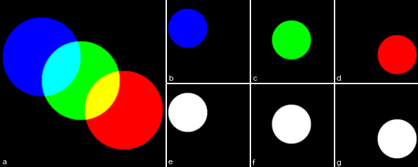
Splitting channels
All the color-spaces mentioned above were constructed using three channels (dimensions). It is a good exercise to visualize each of these channels and realize what they really store, because when I say that the third channel of HSV stores the brightness, what do you expect to see? Remember: a colored image is made of three-channels (in our cases) and when we see each of them separately, what do you think the output will be? If you said a grayscale image, you are correct! However, you might have seen these channels as colored images out there. So, how? For that, we need to choose a fixed value for the other two channels. Let’s do this!
To visualize each channel with color, I used the same values used on the Slides 53 to 65 from CS143, Lecture 03 from Brown University.
RGB or BGR
HSV
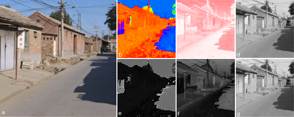
YCrCb or YCbCr
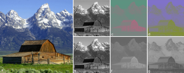
L*a*b or CIE Lab